WeatherNext 3: hourly forecasts on grids as fine as 5 km

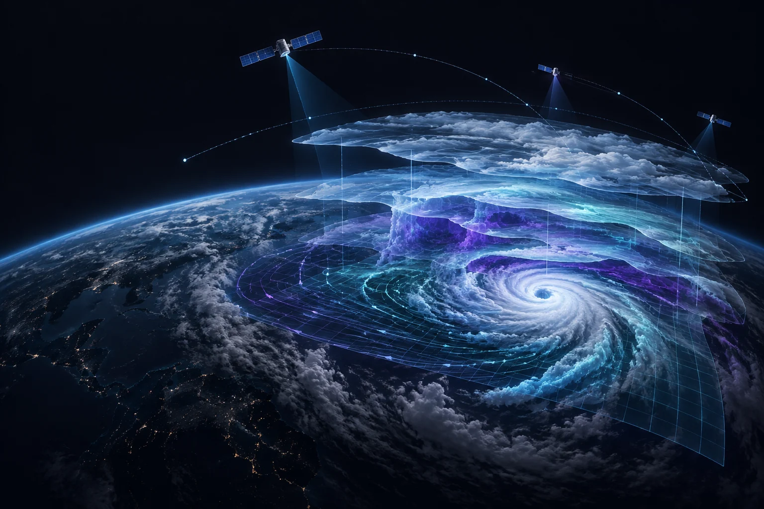
How more frequent forecasting works

WeatherNext 3 combines hourly imagery from geostationary satellites with observations from ground stations and produces a new global forecast every hour. Google reports 5 km grids for key surface variables, 10 km for other surface fields and 25 km for the atmosphere. That is a different cadence from WeatherNext 2, which operated at roughly 25 km resolution and six-hour intervals. The source establishes the system parameters; their operational value still depends on the particular decision, location and weather regime.

The model predicts more than temperature and precipitation. Its outputs include wind at 100 metres, cloud cover and solar radiation, variables that matter when estimating wind and photovoltaic generation. A fresh run can incorporate a newly observed change sooner, but each hourly forecast is not a new direct measurement of the future. It remains a model output. Its usefulness must be evaluated for the relevant horizon and geography, with explicit attention to the consequences of acting on a false alarm or missing an event.

How to interpret the comparisons

Google reports improvements in precipitation CRPS of up to roughly 60% against one reference, around 30% against another and around 10% against a third. Those figures use different comparison systems, so they should not be combined into one universal ranking. CRPS evaluates both the position and the concentration of a probabilistic forecast distribution, with lower values indicating better performance. It is not the percentage of rainy hours predicted correctly, nor a promise of equal improvement in every region.

The phrase “up to 60%” describes the strongest reported difference under a specified comparison. It does not mean that every location, variable and forecast lead time became 60% more accurate. A defensible assessment needs results broken down by region, season, event intensity and horizon. Because the headline findings come from the system’s developer, they should be labelled as Google-reported results. The accompanying paper adds methodological detail, but independent operational evaluation remains a distinct and necessary layer of evidence.

What high resolution does not guarantee

A 5 km grid can represent more local variation than a 25 km grid, but it does not turn every cell into a precise forecast for an individual street. Convective storms, terrain effects and local flows can develop below the model’s resolved scale. A visually detailed output may even create misplaced confidence if users cannot see the spread of plausible scenarios. Spatial resolution is therefore a property of the representation, not sufficient evidence that every local event is predicted accurately.

WeatherNext 3 does not replace national meteorological services or their warning procedures. Official alerts combine multiple models, direct observations, local expertise and institutional accountability. The atmosphere remains chaotic, uncertainty generally grows with lead time, and rare extremes can be especially difficult. The sources support the claim that WeatherNext 3 provides a faster and denser forecasting signal. They do not establish the elimination of surprise errors or complete reliability for safety-critical use.

Turning a forecast into a safer decision

Mateusz’s proposed model separates three layers: the model signal, an operational rule and human accountability. A forecast may indicate a rising risk of reduced renewable generation or intense rainfall. A team should define in advance the threshold at which it checks another source, activates a contingency plan or requests expert review. A consequential decision should not follow from one coloured cell on a map. This is Mateusz’s risk-management framework, not a WeatherNext 3 procedure specified by Google.

The next evidence to watch includes independent results for extreme rainfall, wind and renewable-energy forecasting, together with comparisons spanning complete seasonal cycles. It will also matter whether hourly refreshes improve real decisions rather than only model scores. A useful operational study should measure detected events, false alarms, response delay and the cost of mistakes. Only by connecting probabilistic forecast quality to decision outcomes can researchers show whether the new system creates value beyond a benchmark.

From atmospheric analysis to observation-fed forecasting

The first wave of global AI weather systems learned mainly from meteorological analyses: regular grids estimating the state of the atmosphere by combining observations with a physics-based numerical model. Those grids provide unusually coherent training data, but a model trained on them inherits their latency and biases. The WeatherNext 3 authors report that the operational analysis available to the system can describe a state six to twelve hours old. Its newest geostationary satellite mosaic, by contrast, arrives with less than one hour of latency. The new system does not discard physics or conventional analysis; it adds a much fresher observational channel.

In operation, WeatherNext 3 receives two analysis frames six hours apart and a sequence of recent hourly satellite mosaics. Visible and infrared channels carry information about clouds, water vapour and temperature. The model can therefore refresh a global forecast between the main analysis cycles. This is an architectural shift: machine learning no longer only imitates the finished product of a traditional forecasting system but directly consumes part of the observational stream. It still learns from historical data and remains a model of the atmosphere, however; it is not independently measuring current conditions everywhere.

An ensemble of possibilities, not one certain future

Google’s documentation describes WeatherNext 3 as a 15-day probabilistic model producing 64 ensemble members. Each member is a different model-consistent realization of how the weather could evolve. Their disagreement is not a defect to hide but an approximation of uncertainty arising from both atmospheric chaos and incomplete model knowledge. An ensemble can answer a question about the probability of rainfall or wind crossing a threshold, whereas a single deterministic map shows only one path. That is also why a proper probabilistic score such as CRPS is more informative here than a simple count of correct events.

For a user, the ensemble median, its most dramatic member and a threshold-exceedance probability are three different pieces of information. A utility deciding whether to send a maintenance crew may need a different threshold from someone deciding whether to carry an umbrella. A sound interface should reveal the spread of plausible outcomes and name the rule that turns a forecast into action. Sixty-four members do not guarantee perfect calibration: the ensemble can remain too narrow, and data or architecture errors shared by every member will not be exposed merely by sampling more trajectories.

One network serving several scales and output types

WeatherNext 3 uses an encode–process–decode architecture. Separate encoders map fields at different resolutions onto a shared icosahedral computational mesh, a transformer models their interaction, and decoders produce the required products. Surface temperature, pressure-level atmosphere, precipitation, cyclone tracks and station observations therefore need not be forced into one artificial representation. Hourly surface fields are predicted natively instead of being created later by a separate interpolator between six-hour frames, as they were in the previous generation. This helps explain how one model can serve several forecasting tasks without claiming the same native resolution for every variable.

A separate station head answers a query for an arbitrary place and time by combining the model’s latent state with elevation and land-or-sea metadata. In its production evaluation, Google queried this head on an approximately 0.05-degree grid at hourly intervals. That does not create a measurement at each coordinate: it is still an interpolated model prediction. The distinction matters in valleys, near coasts and across mountainous terrain, where small changes in height or exposure can produce conditions that a global representation cannot fully resolve, however smooth and locally detailed the final map appears.

Evaluation depends on several kinds of ground truth

The authors compare WeatherNext 3 with WeatherNext 2, ECMWF ENS and AIFS ENS, but no single reference can judge every output. Atmospheric fields are evaluated against analyses; temperature and humidity are also checked at stations held out from training; precipitation is compared with satellite products, MRMS radar and rain gauges; and cyclones use best-track records. That is methodologically sensible because no dataset is perfect ground truth for every variable. It also means that every improvement should be read alongside the reference, geography, lead time and resolution-matching procedure used to calculate it.

The principal evaluation covers 2024 with a model trained only through the end of 2023. A further quasi-real-time test ran for six weeks from 1 July to 11 August 2026; the authors caution that this is a small sample and that minor differences should not be over-interpreted. Some comparisons interpolate a lower-resolution forecast onto a finer grid, and the selected reference contributes to the observed advantage. The defensible conclusion is that the paper reports broad improvements in forecast skill, not that it has completed a multi-season operational validation for every region and decision.

Observation gaps and model artifacts remain visible

Surface stations are distributed unevenly. The paper identifies pronounced gaps around the Andes, Himalayas and parts of the high-latitude oceans, where early station-head predictions showed strong biases. The team added pseudo-stations filled with interpolated analysis values to reduce these problems. That is a practical mitigation and a reminder that a global model does not escape the geography of its data. A region with fewer direct measurements may deserve more conservative interpretation even when its map is rendered at exactly the same visual resolution as Europe or North America.

The researchers also show hexagonal patterns inherited from the computational mesh, discontinuities at six-hour boundaries in some station outputs, and under-dispersion in parts of the cyclone-intensity and extent forecasts. These artifacts are weaker in ensemble medians or quantiles than in individual samples, so many downstream uses can remain valuable. They should nevertheless be considered by interfaces and risk models. A finely rendered sample is not automatically a physically coherent scenario, and strong point-wise skill does not guarantee that the full spatial and temporal structure of an event is represented correctly.

A staged curriculum and two kinds of uncertainty

WeatherNext 3 increases the latent width from 768 to 1,024 and the mesh-transformer depth from 24 to 32 layers. The authors did not train the largest configuration at the finest grid from the outset. Their curriculum progressively moved from one degree to 0.25 degrees and then 0.1 degrees, followed by a stage in which the main model was frozen while the station head was fine-tuned. This sequence separates three ideas often collapsed in product descriptions: network capacity, data resolution and the training of a local output head. More transformer layers do not by themselves explain the spatial detail rendered in a forecast product.

The functional-perturbation ensemble is intended to represent both aleatoric uncertainty and uncertainty arising from incomplete model knowledge. Noise in normalization layers handles the first component. WeatherNext 2 used four independently trained seeds for the second, whereas WeatherNext 3 uses two seeds and adds epistemic dropout. At inference, a dropout mask is sampled independently for each ensemble member and time step. The paper presents this as a way to preserve ensemble spread after scaling the model; it is not a general guarantee that every distribution tail or rare event is calibrated correctly. The distinction matters when interpreting 64 trajectories as evidence rather than decoration.

PARDIG and IMERG are not interchangeable labels for rain

The model has separate output heads for two satellite-derived precipitation products. IMERG Final is a widely used NASA dataset that is additionally calibrated against rain gauges. PARDIG is an experimental Google product generated by a separate model trained to predict sparse radar measurements from the GPM core observatory using satellite mosaics and atmospheric fields. Both products use a 0.1-degree grid, but their provenance, availability and error structures differ. Calling both simply “observations” hides an important distinction: one of the training targets is itself a model-derived estimate built from sparse physical measurements.

That difference also shaped the quasi-operational test. IMERG Final did not yet cover July and August 2026, so current precipitation forecasts were evaluated against US MRMS radar and rain gauges. PARDIG achieved the lowest CRPS against MRMS, but the authors emphasize the radar product’s restricted geography and the noise created by a six-week sample. Against rain gauges, the PARDIG and IMERG heads were roughly comparable. This is why a precipitation result must retain the name of its reference product, region and time window rather than collapsing into one generic percentage of “accuracy”.

From forecast to decision: local calibration and action thresholds

A probabilistic forecast is not yet an operational decision. The same signal can mean different things to an electricity-network operator, an event organiser and a municipal response team because the cost of a missed event, the cost of a false alarm and the time available to act are different. A model output should therefore not be translated directly into a universal instruction. The local context comes first: geography, season, forecast horizon, hazard type and the decision the information is meant to support. Only then can a team test whether stated probabilities correspond to observed frequencies under conditions that matter to that particular user.

Local calibration starts by joining archived forecasts to subsequent observations under rules defined in advance. The team examines reliability across horizons and situations, keeping separate results for phenomena that should not be averaged together without justification. Drift also matters: a change in sensors, event definitions, season or the model itself can make an earlier calibration obsolete. A decision interface should consequently show the forecast version, update time, observation source and the domain in which calibration was assessed. One polished score without those boundaries can imply a level of transferability that the evaluation never established.

An action threshold follows from consequences, not from the appearance of a chart. For each decision, the organisation can document which signal triggers monitoring, preparation, intervention or escalation, who authorises the step and when it may be reversed. Candidate thresholds can be replayed against historical cases containing both successful warnings and false alarms, followed by a live exception register after deployment. This arrangement does not remove uncertainty from weather. It turns uncertainty into an explicit, reviewable process in which a forecast informs accountable action without concealing or automatically replacing the judgement behind it.